以下のようなプロットをネット上で見つけました
確か、光学部品を売ってるサイトだったような・・・?
それをそのまま使ってもよかったんですが、chatGPTにその画像と同等のものを作ってもらってみました
結果
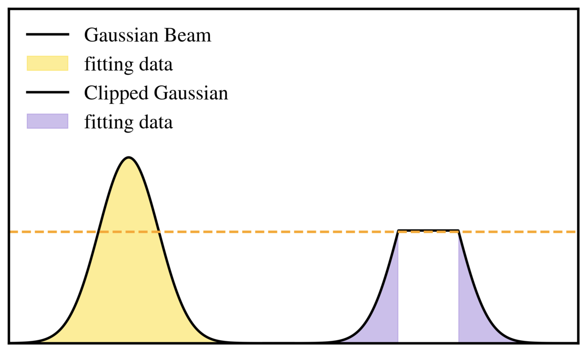
コード例
import numpy as np
import matplotlib.pyplot as plt

import matplotlib as mpl

mpl.rcParams['xtick.labelsize'] = 16
mpl.rcParams['ytick.labelsize'] = 16
mpl.rcParams["axes.labelsize"] = 20
mpl.rcParams["axes.titlesize"] = 20
mpl.rcParams["legend.fontsize"] = 25

mpl.rcParams['axes.linewidth'] = 3

mpl.rcParams['figure.facecolor'] = "white"

mpl.rcParams['mathtext.fontset'] = 'stix'
mpl.rcParams['font.family'] = 'STIXGeneral'


# 軸(ビーム径)
x = np.linspace(-5.5, 5.5, 1600)

# -----------------------------
# 共通の標準偏差 σ
sigma = 1.0

# 左:ガウシアン(正規化して高さ=1)
gauss = np.exp(-x**2 / (2*sigma**2))

# -----------------------------
# 右:ガウシアンをベースにしてクリップ
a = 1  # フラットにする半幅(中心±aまでをクリップ)

# 元のガウス
gauss_raw = np.exp(-x**2 / (2*sigma**2))
H = gauss_raw.max()  # ピーク高さ(=1.0に正規化されている)

# フラット化:中心±a以内をHに置換、それ以外は元のガウス
def clipped_gaussian(x, H=H, a=a, sigma=sigma):
    g = np.exp(-x**2 / (2*sigma**2))
    H = np.exp(-a**2 / (2*sigma**2))
    y = np.where(np.abs(x) <= a, H, g)
    return y

xR = x + 10  # 右へ移動
fgtR = clipped_gaussian(xR-10)

# -----------------------------
# 閾値(しきい値)
thr = 0.6

# -----------------------------
# 描画
plt.figure(figsize=(10,6))

# 左のガウシアン
plt.plot(x, gauss, color='black', label='Gaussian Beam', lw=3)
plt.fill_between(x, 0, gauss, where=(gauss>=0), color='gold', alpha=0.45, label="fitting data")
#plt.fill_between(x, thr, gauss, where=(gauss>thr), color='mediumpurple', alpha=0.35)

# 右のクリップ付きガウス
plt.plot(xR, fgtR, color='black', label='Clipped Gaussian', lw=3)
# plt.fill_between(xR, 0, np.minimum(fgtR, thr), color='gold', alpha=0.45)
# plt.fill_between(xR, thr, fgtR, where=(fgtR>thr), color='mediumpurple', alpha=0.35)
plt.fill_between(xR, 0,  gauss, where=(gauss<=thr), color='mediumpurple', alpha=0.45, label="fitting data")
#plt.fill_between(xR, thr, gauss, where=(gauss>thr), color='mediumpurple', alpha=0.35, label='Excess energy')

# 閾値ライン
plt.axhline(thr, color='orange', ls='--', lw=3)
#plt.text(0.1, thr+0.03, 'Cautery threshold', color='orange')

# 注釈
# plt.text(-2.6, 1.05, 'Gaussian Beam')
# plt.text(5.2, 1.05, 'Clipped Gaussian (Flat top)')
# plt.text(-2.5, 0.33, 'Heating energy')
# plt.text(5.2, 0.33, 'Heating energy')
# plt.text(-0.6, 0.95, 'Excess energy', rotation=38)

# 軸・装飾
#plt.xlabel('Beam Diameter')
plt.yticks([])
plt.xticks([])
plt.ylim(0, 1.8)
plt.xlim(-4, 15)
plt.legend(loc='upper left', frameon=False)
plt.tight_layout()

# 保存・表示
plt.savefig('beam_profile_clipped_gauss.png', dpi=300)
plt.show()